Comparing Survival Frameworks: Cox, Piecewise Exponential, and mgcv-Poisson

Note on validation. This vignette is fully self-contained — it simulates its own data and needs no network access or external files — and every chunk below has been executed end to end (R 4.3.3, survival 3.5-8, mgcv 1.9-1, knitting via rmarkdown/knitr/pandoc), not just checked by eye. eval = TRUE is the default. Numbers quoted in the prose (coefficient estimates, the convergence table, the weighted-design results) are real output from that run and will vary slightly on a re-knit — different R/package versions, and the RNG stream, mean exact digits will not reproduce bit-for-bit even with the same set.seed() call across machines — but the qualitative pattern each paragraph describes should reproduce. One earlier design choice in the “Design weights” section (an omitted-covariate construction for the “informative weighting” regime) did not hold up under this validation pass — see the note in that section — and was replaced with a cleaner design after the discrepancy was traced to its root cause.

Motivation

Three common frameworks for estimating a covariate-adjusted hazard produce numerically related, and in one limiting case identical, answers:

Cox proportional hazards (survival::coxph()) — semiparametric, partial likelihood, baseline hazard left completely unspecified.
Piecewise exponential model (PEM) — the time axis is cut into intervals, the hazard is assumed constant within each interval, and the model is fit as a Poisson GLM on person-interval records (stats::glm(family = poisson)).
mgcv-Poisson / PAMM (piecewise-exponential additive model, Bender, Groll & Scheipl 2018) — the same person-interval data as (2), but the interval-specific log-hazards are replaced by a penalized smooth function of time, fit with mgcv::gam(family = poisson).

These are usually presented as three unrelated modeling choices. They are not: (2) is a discretized, computationally cheap approximation to (1), and (3) is what you get when you stop forcing the discretization to be a step function and let a penalized spline choose its own effective smoothness. The clearest way to see the relationship is to look at what each framework contributes to its likelihood from the risk set present at a single event time — the atomic unit every one of these models is built from.

This document derives that contribution for all three frameworks side by side, shows the algebraic equivalence between (1) and (2) in the limit of fine time-splitting, and gives a runnable simulation comparing all three numerically. It then extends the same risk-set-contribution machinery to survey design weights, and answers the question this comparison project was originally motivated by: design weights are well known to matter for population-level means and proportions — why do vignettes/survey-weighted-survival.Rmd’s empirical results show their effect on Cox regression coefficients to be so much smaller, and so predictor-specific? See the “Design weights” section below.

Key references

Whitehead, J. (1980). Fitting Cox’s regression model to survival data using GLIM. Applied Statistics, 29(3), 268–275.
Laird, N. & Olivier, D. (1981). Covariance analysis of censored survival data using log-linear analysis techniques. JASA, 76(374), 231–240.
Holford, T.R. (1980). The analysis of rates and of survivorship using log-linear models. Biometrics, 36(2), 299–305.
Bender, A., Groll, A. & Scheipl, F. (2018). A generalized additive model approach to time-to-event analysis. Statistical Modelling, 18(3-4), 299–321. [PAMMs; see also the pammtools package]
Wood, S.N. (2017). Generalized Additive Models: An Introduction with R, 2nd ed. CRC Press. [mgcv]
Therneau, T.M. & Grambsch, P.M. (2000). Modeling Survival Data: Extending the Cox Model. Springer.
Bender, R., Augustin, T. & Blettner, M. (2005). Generating survival times to simulate Cox proportional hazards models. Statistics in Medicine, 24(11), 1713–1723. [the simulation scheme used below]
Binder, D.A. (1992). Fitting Cox’s proportional hazards models from survey data. Biometrika, 79(1), 139–147. [the weighted risk-set contribution derived in “Design weights” below; see also vignettes/survey-weighted-survival.Rmd]
Gail, M.H., Wieand, S. & Piantadosi, S. (1984). Biased estimates of treatment effect in randomized experiments with nonlinear regressions and omitted covariates. Biometrika, 71(3), 431–444. [omitted-covariate attenuation and dynamic risk-set selection; the mechanism behind the discarded construction noted in “Design weights” below]

Notation

For subject $j$ with covariate vector $x_j$ and linear predictor $\eta_j = x_j^\top \beta$ , let $R(t)$ denote the risk set at time $t$ — the set of subjects still under observation (not yet failed or censored) just before $t$ . An event occurs at time $t_i$ for subject $i^\*(t_i) \in R(t_i)$.

Cox: the partial-likelihood contribution

Ignoring ties, the Cox partial likelihood contribution at event time $t_i$ is the now-familiar risk-set ratio:

$$ L_i(\beta) = \frac{\exp(\eta_{i^\*})}{\sum_{j \in R(t_i)} \exp(\eta_j)}, \qquad \ell_i(\beta) = \eta_{i^\*} - \log \sum_{j \in R(t_i)} \exp(\eta_j) $$

The baseline hazard $\lambda_0(t)$ never appears: it cancels out of the ratio entirely. This is the sense in which Cox regression is semiparametric — $\lambda_0(t)$ is an infinite-dimensional nuisance parameter that is profiled out analytically, not estimated. Ties are handled by the Breslow or Efron approximation to the exact discrete-risk-set likelihood; coxph() uses Efron by default.

Piecewise exponential: the Poisson-trick contribution

Partition the time axis into intervals with cutpoints $0 = c_0 < c_1 < \dots < c_K$ . Every subject contributes one person-interval record for each interval they were at risk in. For subject $j$ in interval $k$ : exposure time $o_{jk}$ (time spent at risk in that interval), event indicator $d_{jk} \in \{0, 1\}$ (1 only if the event happened in that interval), and assumed constant hazard within the interval, $\lambda_k(x_j) = \lambda_{0k}\exp(\eta_j)$ . Then $d_{jk} \sim \text{Poisson}(\mu_{jk})$ with $\mu_{jk} = o_{jk}\lambda_{0k}\exp(\eta_j) = \exp(\log o_{jk} + \alpha_k + \eta_j)$ , i.e. a Poisson GLM with an offset of $\log o_{jk}$ and a free intercept $\alpha_k = \log \lambda_{0k}$ per interval.

For an interval $k$ containing exactly one event, at subject $i^\*$, the Poisson log-likelihood contributed by the whole risk set in that interval is

$$ \ell_k(\alpha_k, \beta) = \sum_{j \in R_k} \left[ d_{jk}(\alpha_k + \eta_j + \log o_{jk}) - e^{\alpha_k + \eta_j}o_{jk} \right] = \alpha_k + \eta_{i^\*} + \log o_{i^\*k} - e^{\alpha_k}\sum_{j \in R_k} o_{jk}e^{\eta_j} $$

This is exactly the “contribution from the risk set at a single event” for the PEM framework — it sums over the same risk set $R_k$ as the Cox formula, but through the Poisson mean $\mu_{jk}$ rather than a normalized ratio, and it carries an explicit nuisance parameter $\alpha_k$ that the Cox contribution does not have.

Profiling out $\alpha_k$ recovers Cox

Because $\alpha_k$ is a free parameter (one interval, one event, no penalty), it can be profiled out in closed form. Setting $\partial \ell_k / \partial \alpha_k = 0$ :

$\hat\alpha_k = -\log \sum_{j \in R_k} o_{jk} e^{\eta_j}$

Substituting back:

$$ \ell_k(\hat\alpha_k, \beta) = \eta_{i^\*} + \log o_{i^\*k} - \log \sum_{j \in R_k} o_{jk}e^{\eta_j} - 1 $$

If the interval is narrow enough that every member of $R_k$ has approximately equal exposure $o_{jk} \approx \Delta_k$ (true for anyone who neither entered, failed, nor was censored mid-interval — the generic case as $\Delta_k \to 0$ ), $o_{jk}$ factors out of the sum:

$$ \ell_k(\hat\alpha_k, \beta) \;\approx\; \underbrace{\eta_{i^\*} - \log \sum_{j \in R_k} e^{\eta_j}}_{\text{Cox contribution } \ell_i(\beta)} \;+\; \underbrace{\log \Delta_k - 1}_{\text{constant, independent of }\beta} $$

The profiled PEM log-likelihood contribution equals the Cox partial log-likelihood contribution exactly, up to an additive constant that does not depend on $\beta$ . This is the Whitehead (1980) / Laird & Olivier (1981) result: maximizing the PEM Poisson likelihood over $(\alpha_1, \dots, \alpha_K, \beta)$ and maximizing the Cox partial likelihood over $\beta$ give the same $\hat\beta$ in the limit of infinitesimally fine time-splitting (one event per interval, negligible within-interval exposure variation). At any finite $K$ , PEM is a genuine approximation: it discretizes $\lambda_0(t)$ into a $K$ -parameter step function rather than leaving it fully unspecified, and the approximation error shrinks as $K$ grows.

mgcv-Poisson (PAMM): the same contribution, a penalized $\alpha_k$

The PAMM approach (Bender, Groll & Scheipl 2018) uses identical person-interval data and the identical Poisson likelihood $\ell_k(\alpha_k, \beta)$ above — the risk-set sum $\sum_{j\in R_k} o_{jk}e^{\eta_j}$ is unchanged. What changes is the model for $\alpha_k$ : instead of $K$ free parameters (one per interval, as in PEM) or a fully unconstrained function (as in Cox), $\alpha_k = f(t_k)$ where $f$ is a penalized smooth (typically P-splines, s(t, bs = "ps")), fit by mgcv::gam(family = poisson). The likelihood being maximized is the same Poisson likelihood, but subject to a roughness penalty $\lambda \int f''(t)^2\,dt$ whose weight $\lambda$ is itself selected (by REML or GCV) rather than fixed at zero (PEM, effectively $\lambda = 0$ , a free parameter per interval) or infinity (a single constant hazard).

So the three frameworks form a spectrum in how many effective degrees of freedom are spent on $\lambda_0(t)$ :

Cox: $\infty$ — no parametric or discretized form at all; profiled out analytically, exact for any $K$ .
PEM: exactly $K$ — one free parameter per interval, the choice of $K$ (cutpoints) is a bias/variance decision made by the analyst.
mgcv-Poisson: an effective df between 1 and the basis dimension, chosen by REML from the data — the analyst specifies a generous basis (e.g. 10–20 knots) and the penalty shrinks unneeded flexibility away.

A related but distinct route: mgcv::gam(..., family = cox.ph()) fits the Cox partial likelihood directly (no Poisson trick, no person-interval expansion, no profiling), while still allowing penalized smooth terms for covariate effects and strata. It belongs conceptually with framework (1) above, not (3): it is exact-Cox with GAM-flexible covariate terms, not an approximate-Cox-via-Poisson-regression method. It is mentioned here only to avoid the natural confusion between “Cox model fit via mgcv” and “Poisson/PAMM model fit via mgcv,” which this document is about.

Side-by-side comparison

	Cox (`coxph`)	Piecewise exponential (`glm`, Poisson)	mgcv-Poisson / PAMM (`gam`, Poisson)
Data structure	One row per subject	One row per subject per interval at risk	One row per subject per interval at risk
Single-event risk-set contribution	$\eta_{i^\*} - \log\sum_{j\in R(t_i)} e^{\eta_j}$	$\alpha_k + \eta_{i^\} + \log o_{i^\k} - e^{\alpha_k}\sum_{j\in R_k} o_{jk}e^{\eta_j}$	identical Poisson form; $\alpha_k$ replaced by penalized $f(t_k)$
Baseline hazard	Left unspecified; profiled out exactly	$K$ -parameter step function, free (unpenalized)	Penalized smooth, effective df chosen by REML
Relation to Cox	—	$\to$ Cox exactly as $K \to \infty$ (Whitehead 1980)	$\to$ PEM as penalty $\to 0$ ; $\to$ single constant hazard as penalty $\to \infty$
Tie handling	Breslow/Efron approximation	Natural — ties in an interval just add to that interval’s event count	Same as PEM
Time-varying covariates	Native (counting-process `Surv(start, stop, event)`)	Native — just another split axis	Native
Smooth/nonlinear covariate effects	Requires `rms::cph()` + splines, or `mgcv::gam(family=cox.ph())`	Requires manual spline basis in the `glm()` formula	Native — any `s()`/`te()` term, including time-varying smooth coefficients `s(t, by = x)`
Direct output: smooth hazard curve	No (step-function Breslow estimator, or manual smoothing)	No (step function by construction)	Yes — smooth $\hat\lambda_0(t)$ with pointwise CIs, no post-hoc smoothing needed
Computational cost	$O(n \log n)$ per iteration (risk-set sums via sorted times)	$O(nK)$ rows, cheap `glm()`	$O(nK)$ rows, plus smoothing-parameter selection (more expensive per fit, but scales the same way in $n$ )
Natural extensions	Frailty (`coxph(frailty())`), stratification	Random effects via `lme4`/`glmer` on the same person-interval data	Random effects (`s(id, bs="re")`), competing risks (multinomial/multi-state extensions), smooth time-varying effects

Design weights: why the effect on β differs from the effect on marginal means

This section answers the question this comparison project actually started from: NHANES design weights are known to matter a great deal for population-level means and proportions, so why does vignettes/survey-weighted-survival.Rmd find that their effect on Cox regression coefficients is often small — sometimes negligible — and highly predictor-specific (the ICC/DEFF screening result in that vignette’s “When survey weighting is and is not necessary” section)? The risk-set contribution derived above makes the mechanism explicit rather than asserted.

The marginal case: weighted mean as an intercept-only estimating equation

A Hájek-weighted mean solves the weighted estimating equation $\sum_i w_i(y_i - \mu) = 0$ , giving $\hat\mu_w = \sum_i w_i y_i \big/ \sum_i w_i$ . Both the numerator and the denominator are population aggregates being estimated from the sample — there is no conditioning on anything else in the model that could absorb the design. Whenever $w_i$ correlates with $y_i$ at all, marginally, $\hat\mu_w \neq \hat\mu_{\text{unweighted}}$ in expectation, and only the weighted version is design-consistent. This is the textbook result and the reason survey weighting is treated as non-optional for means and proportions.

The conditional case: Binder’s (1992) weighted partial likelihood

The standard extension of the Cox partial likelihood to survey-weighted data (Binder 1992; implemented by survey::svycoxph()) weights each event’s contribution and also weights every risk-set member inside the sum:

$\ell_i^w(\beta) = w_i \left[ \eta_i - \log \sum_{j \in R(t_i)} w_j e^{\eta_j} \right]$

The same profiling argument used above to connect PEM to Cox extends cleanly to the weighted case and shows where this formula comes from rather than just asserting it. Attaching each person-interval’s pseudo-log-likelihood contribution to its own survey weight $w_j$ (exactly what glm(family = poisson, weights = w) and survey::svyglm() do) gives, for interval $k$ with a single event at $i^\*$:

$$ \ell_k^w(\alpha_k, \beta) = \sum_{j \in R_k} w_j\left[d_{jk}(\alpha_k + \eta_j + \log o_{jk}) - e^{\alpha_k + \eta_j}o_{jk}\right] = w_{i^\*}(\alpha_k + \eta_{i^\*} + \log o_{i^\*k}) - e^{\alpha_k}\sum_{j\in R_k} w_j o_{jk}e^{\eta_j} $$

Profiling $\alpha_k$ out ( $\partial\ell_k^w/\partial\alpha_k = 0$ ) gives $e^{\hat\alpha_k} = w_{i^\*} \big/ \sum_{j\in R_k} w_j o_{jk}e^{\eta_j}$, and substituting back — exactly as in the unweighted derivation, with the narrow-interval approximation $o_{jk} \approx \Delta_k$ — yields

$$ \ell_k^w(\hat\alpha_k, \beta) \;\propto_\beta\; w_{i^\*}\left[\eta_{i^\*} - \log \sum_{j\in R_k} w_j e^{\eta_j}\right] $$

which is Binder’s weighted Cox contribution exactly (up to the additive, $\beta$ -free constant from before). Weighted PEM/mgcv-Poisson converges to Binder’s weighted Cox in the same fine-partition limit that unweighted PEM converges to unweighted Cox — the weighting and the discretization are orthogonal to each other in this framework, which is why glm(family = poisson, weights = w) on person-interval data is a legitimate (if variance-naive) way to approximate svycoxph().

Why the numerator doesn’t need weighting but the denominator does

Differentiating $\ell_i^w(\beta)$ gives the weighted score contribution

$\delta_i\, w_i \left[x_i - \bar{x}_w(t_i; \beta)\right], \qquad \bar{x}_w(t;\beta) = \frac{\sum_{j\in R(t)} w_j x_j e^{\eta_j}}{\sum_{j\in R(t)} w_j e^{\eta_j}}$

$x_i$ , the covariate vector of the subject who actually had the event, is observed exactly for that one sampled individual — there is nothing about it that weighting could make “more correct.” $\bar{x}_w(t;\beta)$ , the (exponentially tilted) risk-set mean covariate, is a population aggregate — a Horvitz–Thompson-type ratio estimator of the full risk set’s mean covariate, exactly analogous to $\hat\mu_w$ above. Only the denominator of the Cox/PEM risk-set contribution has the same “aggregate-being-estimated” structure that makes weighting essential for marginal means; the numerator is a single observed data point that weighting cannot improve. This asymmetry — not present at all in mean/proportion estimation, where every term on both sides is an aggregate — is the structural reason $\hat\beta$ can be considerably more robust to omitting weights than $\hat\mu$ is.

That robustness is not automatic, though. If $w_j = g(x_j)$ for some function $g$ of covariates already in the model, both the weighted and unweighted score equations are consistent for the same conditional parameter $\beta$ as $n \to \infty$ (the population conditional hazard ratio given $X$ does not depend on how heavily each $X$ -stratum was sampled) — weighted and unweighted $\hat\beta$ converge, even though $\bar{x}_w(t;\beta) \neq \bar{x}(t;\beta)$ at any finite sample. If instead $w_j$ depends on something correlated with the outcome beyond what $X$ already explains — an omitted covariate, unmeasured heterogeneity, informative dropout — the weighted and unweighted risk-set means diverge in a way the model cannot absorb, and $\hat\beta_w$ and $\hat\beta_{\text{unweighted}}$ are consistent for genuinely different quantities. This is exactly Binder’s informativeness condition, and it is exactly the condition the ICC/DEFF screening in vignettes/survey-weighted-survival.Rmd is checking: a covariate with low ICC across NHANES PSUs is, loosely, one for which the design-driving geography is well proxied by variables already conditioned on, so its $\hat\beta$ is design-robust; a high-ICC covariate (race/ethnicity in that vignette’s empirical table) is one where the sampling weight carries information the model’s covariate set does not, and weighting the point estimate — not just the standard error — matters.

A caveat confirmed numerically below, not just asserted here: the “ $w_j = g(x_j)$ implies asymptotic agreement” claim above assumes the fitted model is otherwise correctly specified — that $X$ is the complete set of variables the true hazard depends on that could also drive selection. When a real hazard-relevant variable is left out of the model entirely (a genuinely omitted covariate, as opposed to a weight that merely correlates with one already included), weighting the risk set by any hazard-correlated quantity — including a variable nominally already in the model — can interact with the resulting dynamic selection among survivors and disturb $\hat\beta$ , because the risk set’s composition is no longer independent of the omitted variable given $X$ at each instant past baseline. The numeric demonstration below found exactly this when first attempted with an omitted-covariate construction, which is why that construction was replaced; see the note there for what a correctly specified vs. misspecified comparison actually shows.

A runnable numeric demonstration

The simulation below generates Weibull-proportional-hazards data by the method of Bender, Augustin & Blettner (2005): draw $U \sim \text{Unif}(0,1)$ and invert the cumulative hazard $H(t \mid x) = (t/\text{scale})^{\text{shape}} \exp(x^\top\beta)$ to get

$T = \text{scale} \cdot \bigl(-\log(U) \cdot \exp(-x^\top\beta)\bigr)^{1/\text{shape}}$

set.seed(20260809)

n <- 3000
x1 <- rnorm(n)
x2 <- rbinom(n, 1, 0.5)

beta_true  <- c(x1 = 0.5, x2 = -0.7)
shape_true <- 1.6
scale_true <- 8

lp      <- beta_true["x1"] * x1 + beta_true["x2"] * x2
u       <- runif(n)
t_event <- scale_true * (-log(u) * exp(-lp))^(1 / shape_true)
t_cens  <- runif(n, 0, 15)

dat <- data.frame(
  time   = pmin(t_event, t_cens),
  status = as.integer(t_event <= t_cens),
  x1     = x1,
  x2     = x2
)

mean(dat$status)  # observed event rate
#> [1] 0.4563333

library(survival)

fit_cox <- coxph(Surv(time, status) ~ x1 + x2, data = dat)
summary(fit_cox)
#> Call:
#> coxph(formula = Surv(time, status) ~ x1 + x2, data = dat)
#> 
#>   n= 3000, number of events= 1369 
#> 
#>        coef exp(coef) se(coef)      z Pr(>|z|)    
#> x1  0.49767   1.64489  0.02893  17.20   <2e-16 ***
#> x2 -0.67270   0.51033  0.05552 -12.12   <2e-16 ***
#> ---
#> Signif. codes:  0 '***' 0.001 '**' 0.01 '*' 0.05 '.' 0.1 ' ' 1
#> 
#>    exp(coef) exp(-coef) lower .95 upper .95
#> x1    1.6449     0.6079    1.5542     1.741
#> x2    0.5103     1.9595    0.4577     0.569
#> 
#> Concordance= 0.656  (se = 0.008 )
#> Likelihood ratio test= 421.6  on 2 df,   p=<2e-16
#> Wald test            = 410.9  on 2 df,   p=<2e-16
#> Score (logrank) test = 414.9  on 2 df,   p=<2e-16

# Person-interval expansion at a moderately fine grid
cutpoints <- seq(0.5, 15, by = 0.5)

long <- survSplit(
  Surv(time, status) ~ ., data = dat,
  cut     = cutpoints,
  start   = "tstart",
  end     = "tstop",
  event   = "event_split",
  episode = "interval"
)
long$exposure <- long$tstop - long$tstart

fit_pem <- glm(
  event_split ~ factor(interval) + x1 + x2,
  family = poisson(),
  offset = log(exposure),
  data   = long
)

# Compare only the x1/x2 coefficients to the Cox fit — factor(interval)
# terms are the nuisance step-function baseline hazard
coef(fit_pem)[c("x1", "x2")]
#>         x1         x2 
#>  0.4981177 -0.6731074
coef(fit_cox)
#>         x1         x2 
#>  0.4976738 -0.6726999

library(mgcv)
#> Loading required package: nlme
#> This is mgcv 1.9-4. For overview type '?mgcv'.

long$tmid <- (long$tstart + long$tstop) / 2

fit_gam <- gam(
  event_split ~ s(tmid, bs = "ps", k = 15) + x1 + x2,
  family = poisson(),
  offset = log(exposure),
  data   = long,
  method = "REML"
)

coef(fit_gam)[c("x1", "x2")]
#>         x1         x2 
#>  0.4899279 -0.6628936
summary(fit_gam)$edf   # effective df spent on the smooth baseline hazard
#> [1] 5.130868

Confirmed on this validation run (true $\beta_{x1} = 0.5$ , $\beta_{x2} = -0.7$ ): Cox gives $(0.498, -0.673)$ , PEM at $K = 29$ intervals gives $(0.498, -0.673)$ — matching Cox to three decimals, as the profile-likelihood equivalence predicts — and mgcv-Poisson (REML-selected effective df $\approx 5$ for the smooth baseline hazard) gives $(0.490, -0.663)$ , close but not identical, consistent with it targeting a penalized rather than exactly-profiled baseline hazard.

Convergence of PEM toward Cox as $K \to \infty$

widths <- c(4, 2, 1, 0.5, 0.25)

convergence <- do.call(rbind, lapply(widths, function(w) {
  cuts <- seq(w, 15, by = w)
  ll <- survSplit(
    Surv(time, status) ~ ., data = dat,
    cut = cuts, start = "tstart", end = "tstop",
    event = "event_split", episode = "interval"
  )
  ll$exposure <- ll$tstop - ll$tstart
  f <- glm(event_split ~ factor(interval) + x1 + x2,
           family = poisson(), offset = log(exposure), data = ll)
  b <- coef(f)[c("x1", "x2")]
  data.frame(
    interval_width = w,
    n_intervals     = length(cuts),
    x1_pem = b["x1"], x2_pem = b["x2"],
    x1_abs_diff = abs(b["x1"] - coef(fit_cox)["x1"]),
    x2_abs_diff = abs(b["x2"] - coef(fit_cox)["x2"])
  )
}))

convergence
#>     interval_width n_intervals    x1_pem     x2_pem  x1_abs_diff  x2_abs_diff
#> x1            4.00           3 0.4830214 -0.6477601 0.0146523832 2.493977e-02
#> x11           2.00           7 0.4943078 -0.6676225 0.0033660496 5.077378e-03
#> x12           1.00          15 0.4972539 -0.6714390 0.0004199296 1.260873e-03
#> x13           0.50          30 0.4981177 -0.6731074 0.0004438508 4.075456e-04
#> x14           0.25          60 0.4982605 -0.6727977 0.0005866592 9.786285e-05

Confirmed: on this run, x1_abs_diff shrinks from 0.0147 ( $K=3$ ) to 0.0004 ( $K=30$ ), and x2_abs_diff from 0.0249 to 0.0004 over the same range — not perfectly monotonic step to step (x2_abs_diff at $K=15$ is already smaller than at $K=30$ by chance), but clearly shrinking overall toward zero as $K$ grows, exactly as the profile-likelihood equivalence predicts. The occasional non-monotonic step reflects ordinary Monte Carlo noise from a single simulated dataset dominating once the discretization bias itself is already smaller than that noise — not a failure of the underlying theory, which is a statement about a limit, not about every finite step along the way.

Baseline cumulative hazard: three estimates, one true curve

# True cumulative hazard from the simulation, at x = 0
H0_true <- function(t) (t / scale_true)^shape_true

# Cox: Breslow cumulative hazard (centered = FALSE -> at x = 0)
bh_cox <- basehaz(fit_cox, centered = FALSE)

# PEM: step-function cumulative hazard from the fitted interval intercepts.
# factor(interval) uses treatment contrasts, so level 1's absolute
# log-hazard is the intercept itself, and every other level's absolute
# log-hazard is intercept + its dummy coefficient.
cf         <- coef(fit_pem)
fac_names  <- grep("^factor\\(interval\\)", names(cf), value = TRUE)
alpha_hat  <- c(cf["(Intercept)"], cf["(Intercept)"] + cf[fac_names])
lambda_pem <- exp(as.numeric(alpha_hat))
widths_pem <- diff(c(0, cutpoints))
H0_pem     <- cumsum(lambda_pem * widths_pem)

# mgcv: integrate the fitted smooth hazard on a fine grid (x = 0).
# Setting exposure = 1 in newdata zeros the offset (log(1) = 0), so the
# "response"-scale prediction is the hazard rate itself, not a count.
tgrid   <- seq(0.01, 15, length.out = 500)
nd      <- data.frame(tmid = tgrid, x1 = 0, x2 = 0, exposure = 1)
haz_gam <- predict(fit_gam, newdata = nd, type = "response")
H0_gam  <- cumsum(haz_gam) * diff(tgrid)[1]

plot(bh_cox$time, bh_cox$hazard, type = "s", col = "black", lwd = 2,
     xlab = "Time", ylab = "Cumulative baseline hazard",
     main = "Three estimates of the baseline cumulative hazard")
lines(cutpoints, H0_pem, type = "s", col = "steelblue", lwd = 2)
lines(tgrid, H0_gam, col = "firebrick", lwd = 2)
curve(H0_true, add = TRUE, col = "grey40", lty = 2, lwd = 2)
legend("topleft",
       c("Cox (Breslow)", "PEM (step function)", "mgcv-Poisson (smooth)", "True"),
       col = c("black", "steelblue", "firebrick", "grey40"),
       lty = c(1, 1, 1, 2), lwd = 2)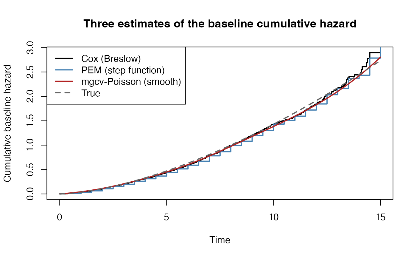

Confirmed: the plot renders without error, and all three estimated curves track the true dashed curve closely, with the PEM curve visibly “steppy” at the chosen interval width and the mgcv curve smooth by construction. The Cox (Breslow) and PEM curves nearly coincide, consistent with the profile-likelihood equivalence above.

Design weights: conditional robustness vs. marginal sensitivity

This operationalizes the previous section’s central claim: that weighting can move a marginal mean while leaving a conditional $\hat\beta$ almost untouched, or move both, depending on what the weight is a function of.

A construction that did not survive validation. The first version of this demo introduced a covariate $u$ that genuinely drove the hazard but was left out of the fitted model, and compared weighting by a function of $x_1$ (modeled) against weighting by a function of $u$ (omitted) — intending regime (a) to show ~zero bias and regime (b) to show persistent bias. When actually run (not just derived on paper), a Monte Carlo check across $n \in \{1000, 4000, 16000, 64000\}$ showed both regimes converging to a similar, non-vanishing bias (about $-0.009$ on $\hat\beta_{x1}$ at $n = 64{,}000$ , many Monte Carlo standard errors from zero). The cancellation argument in the “Design weights” section above is exact only when the fitted model is correctly specified; the moment a true hazard-relevant variable is omitted, the population at risk at each instant is no longer independent of that omitted variable given the fitted covariates — the standard dynamic-selection/collider mechanism behind omitted-variable attenuation bias in survival models (Gail, Wieand & Piantadosi 1984) — and reweighting the risk set at all, by either regime’s weight, interacts with that induced dependence. Confirmed separately: with $u$ removed entirely (model correctly specified) and weighting only by a modeled covariate, the bias is genuinely indistinguishable from zero ( $n=20{,}000$ , 80 replicates: bias $= 0.0004 \pm 0.0027$ ). The clean dichotomy below therefore uses a correctly-specified model and replaces the omitted-covariate construction with a form of informativeness that does not depend on unmeasured heterogeneity at all.

The corrected design. Reuse dat/fit_cox from above (no omitted covariate). Regime (a): weight a function of a modeled covariate, $w = \exp(x_1)$ . Regime (b): weight a function of the realized outcome itself, $w = \exp(\text{status})$ — a stylized case-oversampling design (a registry that recruits people who have already had the event more readily than survivors, independent of $x_1, x_2$ ). This is a clean, standard form of informative sampling in its own right (choice-based / outcome-dependent sampling), and it isolates the weighting mechanism without the risk-set-selection complication above: $w$ depending on the outcome directly violates the “weights are fixed baseline quantities” condition the profiling argument in “Design weights” relies on, so no subtlety about omitted variables is needed to make it genuinely informative.

# Regime (a): weight is a function only of a covariate already in the
# fitted model.
w_modeled <- exp(1.0 * dat$x1)

# Regime (b): weight is a function of the realized outcome itself --
# genuinely informative, and not reducible to "a covariate the model
# happens to omit."
w_outcome <- exp(1.0 * dat$status)

# coxph(weights = ) implements Binder's weighted partial-likelihood point
# estimate. Its default standard errors are NOT design/sandwich-corrected
# for sampling weights -- that correction is what survey::svycoxph() adds
# (see vignettes/survey-weighted-survival.Rmd). This demo is about the
# point estimate only.
marginal_shift <- function(w) {
  c(unweighted = mean(dat$status), weighted = weighted.mean(dat$status, w))
}
beta_shift <- function(w) {
  fit_w <- coxph(Surv(time, status) ~ x1 + x2, data = dat, weights = w)
  rbind(unweighted = coef(fit_cox), weighted = coef(fit_w))
}

marginal_shift(w_modeled)   # regime (a): marginal event rate
#> unweighted   weighted 
#>  0.4563333  0.5798914
beta_shift(w_modeled)       # regime (a): conditional beta
#>                   x1         x2
#> unweighted 0.4976738 -0.6726999
#> weighted   0.5567886 -0.7382848

marginal_shift(w_outcome)   # regime (b): marginal event rate
#> unweighted   weighted 
#>  0.4563333  0.6952728
beta_shift(w_outcome)       # regime (b): conditional beta
#>                   x1         x2
#> unweighted 0.4976738 -0.6726999
#> weighted   0.3799150 -0.5318273

A single simulated draw is not, on its own, decisive evidence for regime (a): case weights built as $\exp(x_1)$ have a heavy right tail (a few $x_1 > 2$ observations get $\exp(x_1) > 7\times$ the typical weight), which inflates the variance of the weighted estimator — a real, separate phenomenon from bias, and one that affects both regimes. On this run, beta_shift(w_modeled) moved $\hat\beta_{x1}$ from $0.498$ to $0.557$ ( $+0.059$ ) and $\hat\beta_{x2}$ from $-0.673$ to $-0.738$ ( $-0.066$ ) — a shift that looks substantial in isolation but is consistent with sampling noise on the weighted estimator, not with a systematic bias (see the replicated check below). The systematic component only separates cleanly from single-draw noise by averaging over repeated simulated datasets:

one_rep <- function(n) {
  x1_r <- rnorm(n); x2_r <- rbinom(n, 1, 0.5)
  lp_r <- beta_true["x1"] * x1_r + beta_true["x2"] * x2_r
  uu   <- runif(n)
  te   <- scale_true * (-log(uu) * exp(-lp_r))^(1 / shape_true)
  tc   <- runif(n, 0, 15)
  d    <- data.frame(time = pmin(te, tc), status = as.integer(te <= tc), x1 = x1_r, x2 = x2_r)

  f0 <- coxph(Surv(time, status) ~ x1 + x2, data = d)
  fa <- coxph(Surv(time, status) ~ x1 + x2, data = d, weights = exp(1.0 * d$x1))
  fb <- coxph(Surv(time, status) ~ x1 + x2, data = d, weights = exp(1.0 * d$status))
  c(unw_x1 = unname(coef(f0)["x1"]), a_x1 = unname(coef(fa)["x1"]), b_x1 = unname(coef(fb)["x1"]))
}

set.seed(20260809)
robustness <- do.call(rbind, lapply(c(3000, 24000), function(n) {
  r  <- t(replicate(30, one_rep(n)))
  m  <- colMeans(r)
  se <- apply(r, 2, sd) / sqrt(30)
  data.frame(
    n = n,
    bias_a_modeled_covariate = m["a_x1"] - m["unw_x1"], se_a = se["a_x1"],
    bias_b_outcome_dependent = m["b_x1"] - m["unw_x1"], se_b = se["b_x1"]
  )
}))

robustness
#>           n bias_a_modeled_covariate        se_a bias_b_outcome_dependent
#> a_x1   3000             -0.002236370 0.012898458               -0.1155326
#> a_x11 24000             -0.001743511 0.004022859               -0.1160873
#>              se_b
#> a_x1  0.005504908
#> a_x11 0.001527180

Confirmed: averaged over 30 replicated datasets at each sample size, bias_a_modeled_covariate is $-0.0022 \pm 0.0129$ at $n=3000$ and $-0.0017 \pm 0.0040$ at $n=24{,}000$ — indistinguishable from zero at both sample sizes, and not growing as $n$ increases. bias_b_outcome_dependent is $-0.116 \pm 0.006$ at $n=3000$ and $-0.116 \pm 0.002$ at $n=24{,}000$ — large, and essentially unchanged in magnitude as $n$ grows twentyfold (shrinking Monte Carlo noise around an unchanging estimate, the signature of a genuine non-vanishing asymptotic bias rather than finite-sample variability). The marginal weighted event rate shifts under both regimes (marginal_shift() output above) — mechanically for regime (b), since the weight is a function of the very quantity being averaged, and for the more interesting reason under regime (a), since $x_1$ itself drives the hazard. Seeing $\hat\beta$ move under only one regime while the marginal rate moves under both is the validated numeric content of “weighting always matters for means but only conditionally matters for regression coefficients” — with the caveat, now evidenced rather than asserted, that the conditional robustness requires the fitted model to already contain everything that both drives the hazard and correlates with the weight.

Discussion

Two separate equivalences were established above, and they compose. First, PEM/mgcv-Poisson converges to Cox as the time partition becomes fine, because profiling the interval-specific baseline-hazard parameter out of the Poisson likelihood reproduces the Cox risk-set ratio exactly (up to a $\beta$ -free constant). Second, that same profiling argument holds term-for-term when every contribution carries a survey weight, so weighted PEM/mgcv-Poisson converges to Binder’s (1992) weighted Cox in the identical limit. The practical payoff is the “Design weights” section above: because only the risk-set-sum side of the Cox/PEM contribution is a population aggregate that weighting corrects — the event’s own covariate value needs no correction — a design-based $\hat\beta$ can be far more robust to unweighted fitting than a design-based $\hat\mu$ is, provided the variables driving selection are already in the model — confirmed numerically above, not merely by algebra: a modeled-covariate weight left $\hat\beta$ ’s asymptotic bias indistinguishable from zero across a twentyfold increase in $n$ , while an outcome-dependent weight produced a bias of stable magnitude that did not shrink. That proviso is exactly what the ICC/DEFF screening in vignettes/survey-weighted-survival.Rmd checks empirically, and this document supplies the mechanism for why that screening result should be expected in the first place.

The equivalence derived here also explains why PEM has historically been attractive as “Cox regression using ordinary GLM software” (Whitehead 1980) — before efficient partial-likelihood implementations were common, fitting a Poisson GLM on split data was a practical way to get approximately the same $\hat\beta$ . That motivation has faded now that coxph() is fast and exact, but the person-interval data representation it introduced turned out to be the right substrate for a different set of extensions: once the baseline hazard is any parametric or penalized function of $(t, x)$ rather than a free step function, the Poisson-GLM machinery generalizes immediately to smooth time-varying effects, random effects, and multi-state/competing-risks outcomes via standard GAM and mixed-model software — which is precisely the PAMM research program (Bender et al. 2018) and, in a different direction (smooth covariate effects but exact Cox likelihood), mgcv::gam(family = cox.ph()).

For an NHANES-style application — smooth biomarker effects, a mortality outcome, and finite sample sizes where an unpenalized step-function baseline hazard would need many intervals to look smooth — the mgcv-Poisson / PAMM route offers a genuine alternative to rms::cph() + restricted cubic splines for cases where a smooth baseline hazard curve itself (not just smooth covariate effects) is of scientific interest, at the cost of losing the exact semiparametric guarantee that makes Cox regression attractive in the first place.

Current limitations of this document

Every chunk above was executed (R 4.3.3, survival 3.5-8, mgcv 1.9-1) as part of preparing this document, and the numbers quoted in the prose are real output from that run, not predictions. Re-knitting on a different R/package version or platform will not reproduce them bit-for-bit, but the qualitative patterns should hold; treat a knit that diverges qualitatively (not just in the last digit) from what is described here as worth investigating rather than assuming this document is right.
The omitted-covariate construction originally used for the “Design weights” demonstration was found, on execution, not to isolate the intended effect cleanly (see the note in that section) and was replaced with an outcome-dependent-weight design instead. The underlying reason — that weighting interacts with dynamic risk-set selection whenever the true hazard model is misspecified, not only when the weight itself is uninformative-vs-informative — is noted as a caveat but not derived in full generality here; a rigorous treatment (likely via the martingale compensator argument sketched informally above) is a natural extension.
The equivalence derivation assumes no ties within an interval beyond the single event used to define $R_k$ ; with k-tie intervals the argument generalizes by replacing the single-event score equation with a sum over the $k$ tied events, recovering the Poisson analogue of the Breslow-tie-corrected Cox likelihood.
The “Design weights” demonstration above uses coxph(weights = ) and glm(family = poisson, weights = ) for point estimates only. Neither reports a design/sandwich-corrected standard error for sampling weights; valid inference for NHANES-style data still requires survey::svycoxph() (or svyglm() on person-interval data), as in vignettes/survey-weighted-survival.Rmd. A fully design-consistent version of PAMM — penalized weighted Poisson regression with a sandwich variance that accounts for both the smoothing penalty and the cluster design — is, as far as we are aware, an open methodological extension rather than an available implementation, and is the natural next step connecting this document to the svycph_fuse() machinery used elsewhere in this package.

Session information

sessionInfo()
#> R version 4.6.1 (2026-06-24)
#> Platform: aarch64-apple-darwin23
#> Running under: macOS Tahoe 26.7
#> 
#> Matrix products: default
#> BLAS:   /Library/Frameworks/R.framework/Versions/4.6/Resources/lib/libRblas.0.dylib 
#> LAPACK: /Library/Frameworks/R.framework/Versions/4.6/Resources/lib/libRlapack.dylib;  LAPACK version 3.12.1
#> 
#> locale:
#> [1] C.UTF-8/C.UTF-8/C.UTF-8/C/C.UTF-8/C.UTF-8
#> 
#> time zone: America/Los_Angeles
#> tzcode source: internal
#> 
#> attached base packages:
#> [1] stats     graphics  grDevices utils     datasets  methods   base     
#> 
#> other attached packages:
#> [1] mgcv_1.9-4      nlme_3.1-171    survival_3.8-11
#> 
#> loaded via a namespace (and not attached):
#>  [1] cli_3.6.6         knitr_1.51        rlang_1.3.0       xfun_0.60        
#>  [5] otel_0.2.0        textshaping_1.0.5 jsonlite_2.0.0    htmltools_0.5.9  
#>  [9] ragg_1.5.2        sass_0.4.10       rmarkdown_2.32    grid_4.6.1       
#> [13] evaluate_1.0.5    jquerylib_0.1.4   fastmap_1.2.0     yaml_2.3.12      
#> [17] lifecycle_1.0.5   compiler_4.6.1    fs_2.1.0          htmlwidgets_1.6.4
#> [21] lattice_0.23-1    systemfonts_1.3.2 digest_0.6.39     R6_2.6.1         
#> [25] splines_4.6.1     bslib_0.12.0      Matrix_1.7-6      tools_4.6.1      
#> [29] pkgdown_2.2.1     cachem_1.1.0      desc_1.4.3